3. Getting started with prenspire

import random
from pathlib import Path

import lmfit
import numpy as np

from clophfit import prenspire
from clophfit.fitting.core import (
    DataArray,
    Dataset,
    analyze_spectra,
    analyze_spectra_glob,
    fit_binding_glob,
    weight_multi_ds_titration,
)
from clophfit.fitting.plotting import plot_emcee

%load_ext autoreload
%autoreload 2
tpath = Path("../../tests/EnSpire")

ef1 = prenspire.EnspireFile(tpath / "h148g-spettroC.csv")
ef2 = prenspire.EnspireFile(tpath / "e2-T-without_sample_column.csv")
ef3 = prenspire.EnspireFile(tpath / "24well_clop0_95.csv")

ef3.wells, ef3._wells_platemap, ef3._platemap

(['A03', 'A04', 'A05', 'A06', 'B01', 'B02', 'C01', 'C02', 'C03'],
 ['A03', 'A04', 'A05', 'A06', 'B01', 'B02', 'C01', 'C02', 'C03'],
 [['A', '  ', '  ', '- ', '- ', '- ', '- '],
  ['B', '- ', '- ', '  ', '  ', '  ', '  '],
  ['C', '- ', '- ', '- ', '  ', '  ', '  '],
  ['D', '  ', '  ', '  ', '  ', '  ', '  ']])

ef1.__dict__.keys()

dict_keys(['file', 'verbose', 'metadata', 'measurements', 'wells', '_ini', '_fin', '_wells_platemap', '_platemap'])

ef1.measurements.keys(), ef2.measurements.keys()

(dict_keys(['A']), dict_keys(['B', 'A', 'C', 'D', 'E', 'F', 'G', 'H']))

when testing each spectra for the presence of a single wavelength in the appropriate monochromator

ef2.measurements["A"]["metadata"]

{'temp': '25',
 'Monochromator': 'Excitation',
 'Min wavelength': '400',
 'Max wavelength': '510',
 'Wavelength': '530',
 'Using of excitation filter': 'Top',
 'Measurement height': '8.9',
 'Number of flashes': '50',
 'Number of flashes integrated': '50',
 'Flash power': '100'}

ef2.measurements["A"].keys()

dict_keys(['metadata', 'lambda', 'F01', 'F02', 'F03', 'F04', 'F05', 'F06', 'F07'])

random.seed(11)
random.sample(ef1.measurements["A"]["F01"], 7)

[2163.0, 607.0, 1846.0, 517.0, 572.0, 2145.0, 2028.0]

fp = tpath / "h148g-spettroC-nota.csv"
n1 = prenspire.Note(fp, verbose=1)
n1._note.set_index("Well").loc["A01", ["Name", "Temp"]]

Wells ['A01', 'A02']...['G04', 'G05'] generated.

Name    H148G
Temp     20.0
Name: A01, dtype: object

n1.__dict__.keys()

dict_keys(['fpath', 'verbose', 'wells', '_note', 'titrations'])

n1.wells == ef1.wells, n1.wells == ef2.wells

(True, False)

n1.build_titrations(ef1)
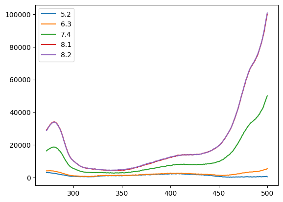
tit0 = n1.titrations["H148G"][20.0]["Cl_0.0"]["A"]
tit3 = n1.titrations["H148G"][20.0]["pH_7.4"]["A"]
tit0

	5.2	6.3	7.4	8.1	8.2
272.0	3151.0	4181.0	16413.0	29192.0	28816.0
273.0	3130.0	4204.0	16926.0	29909.0	29545.0
274.0	3043.0	4232.0	17331.0	30900.0	30750.0
275.0	3079.0	4283.0	17680.0	31717.0	31547.0
276.0	2975.0	4264.0	18020.0	32564.0	32336.0
...	...	...	...	...	...
496.0	636.0	4689.0	43230.0	87203.0	87842.0
497.0	683.0	4923.0	45173.0	89719.0	90666.0
498.0	632.0	4900.0	46725.0	93452.0	94101.0
499.0	854.0	5140.0	48452.0	96643.0	97506.0
500.0	573.0	5573.0	50025.0	99847.0	100715.0

229 rows × 5 columns

tit0.plot()
tit3.plot()

<Axes: >

ef = prenspire.EnspireFile(tpath / "G10.csv")
fp = tpath / "NTT-G10_note.csv"
nn = prenspire.Note(fp, verbose=1)
nn.build_titrations(ef)
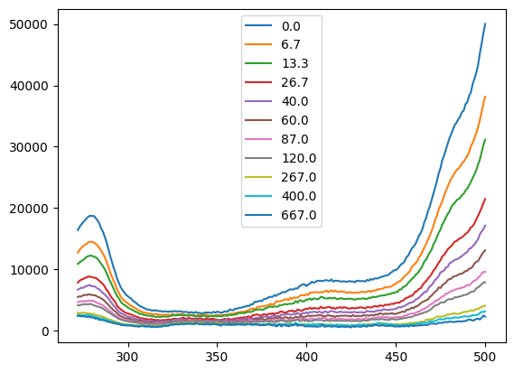
spectra = nn.titrations["NTT-G10"][20.0]["Cl_0.0"]["C"]

Wells ['D01', 'D02']...['G07', 'G08'] generated.

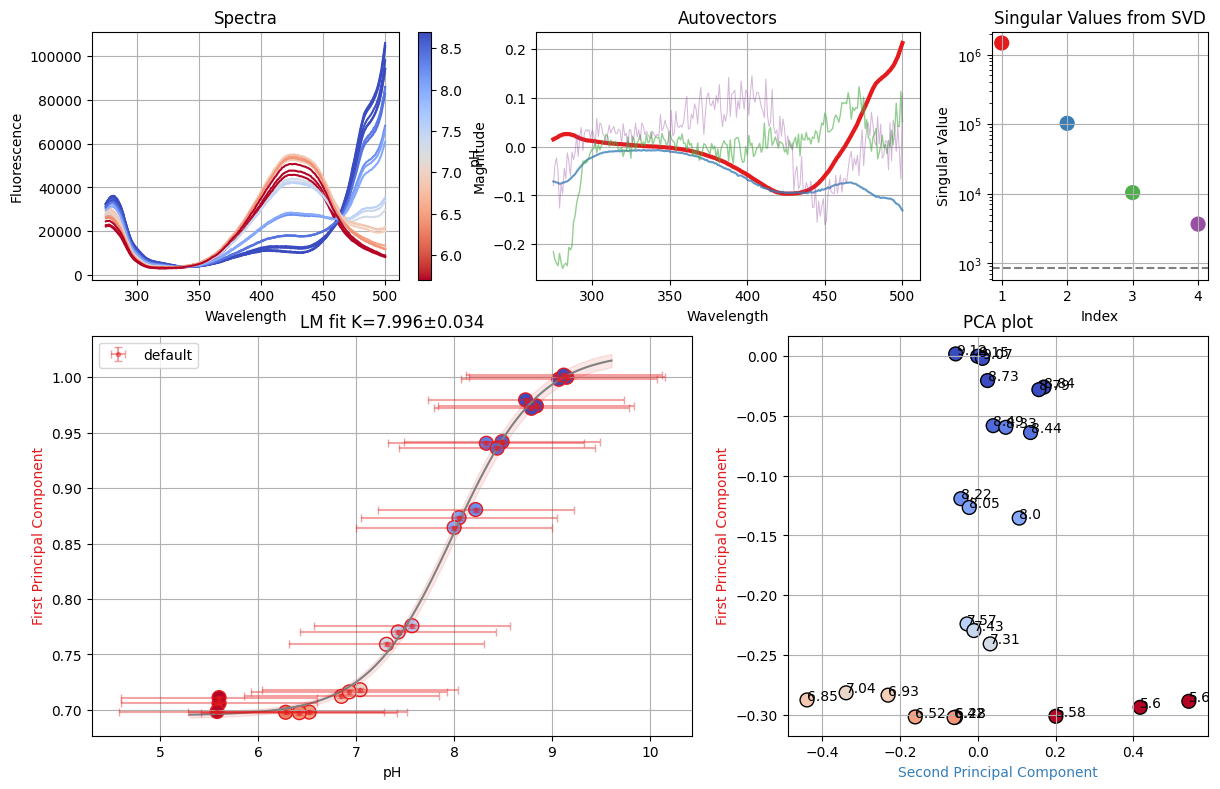
f_res = analyze_spectra(spectra, is_ph=True, band=None)
print(f_res.result.chisqr)
f_res.figure

551.9999999926993

def dataset_from_lres(lkey, lres, is_ph):
    data = {}
    for k, res in zip(lkey, lres, strict=False):
        x = res.mini.userargs[0]["default"].x
        y = res.mini.userargs[0]["default"].y
        data[k] = DataArray(x, y)
    return Dataset(data, is_ph=is_ph)


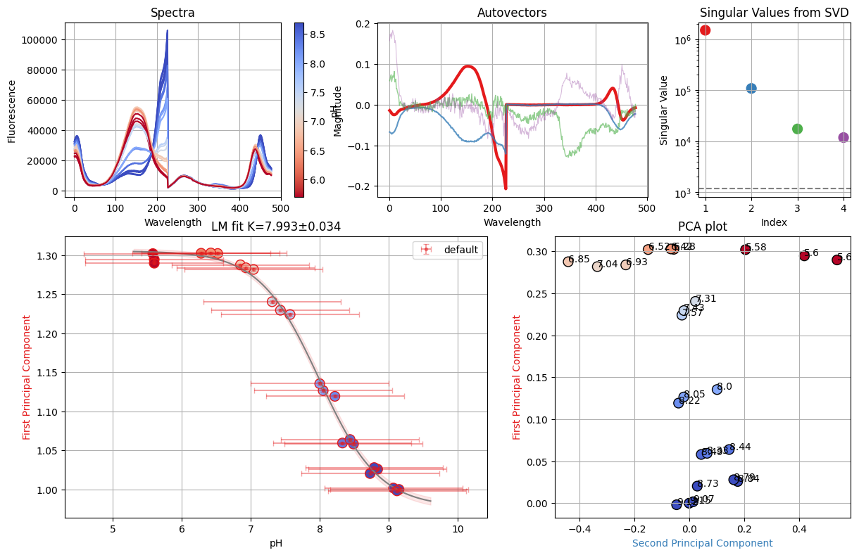
spectra_A = nn.titrations["NTT-G10"][20.0]["Cl_0.0"]["A"]
spectra_C = nn.titrations["NTT-G10"][20.0]["Cl_0.0"]["C"]
spectra_D = nn.titrations["NTT-G10"][20.0]["Cl_0.0"]["D"]

resA = analyze_spectra(spectra_A, is_ph=True, band=(466, 510))
resC = analyze_spectra(spectra_C, is_ph=True, band=(470, 500))
resD = analyze_spectra(spectra_D, is_ph=True, band=(450, 600))

ds_bands = dataset_from_lres(["A", "C", "D"], [resA, resC, resD], is_ph=True)

resA = analyze_spectra(spectra_A, is_ph=True)
resC = analyze_spectra(spectra_C, is_ph=True)
resD = analyze_spectra(spectra_D, is_ph=True)
ds_svd = dataset_from_lres(["A", "C", "D"], [resA, resC, resD], is_ph=True)

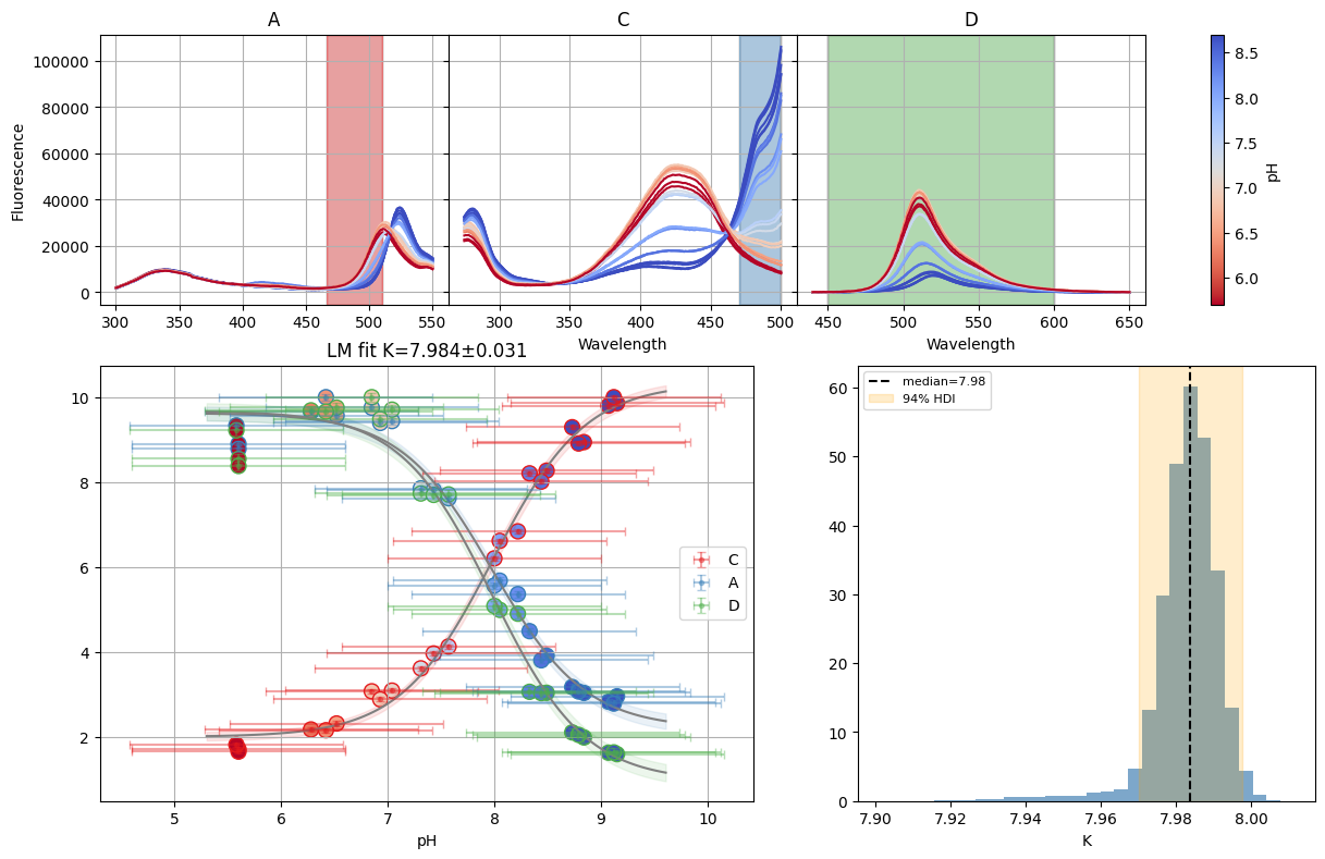
dbands = {"D": (466, 510)}
tit = nn.titrations["NTT-G10"][20.0]["Cl_0.0"]
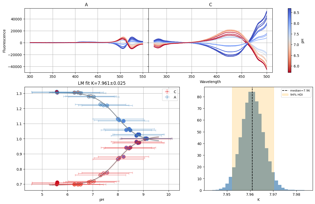
sgres = analyze_spectra_glob(tit, ds_svd, dbands)

sgres.svd.figure

The chain is shorter than 50 times the integrated autocorrelation time for 1 parameter(s). Use this estimate with caution and run a longer chain!
N/50 = 108;
tau: [ 40.20896098  96.52905818 108.39902902  56.17331176  41.31462928]

sgres.gsvd.figure

dbands = {"A": (466, 510), "C": (470, 500), "D": (450, 600)}
sgres = analyze_spectra_glob(nn.titrations["NTT-G10"][20.0]["Cl_0.0"], ds_bands, dbands)
sgres.bands.figure

The chain is shorter than 50 times the integrated autocorrelation time for 5 parameter(s). Use this estimate with caution and run a longer chain!
N/50 = 108;
tau: [194.05196729 251.44260563  52.89323644 170.71290562 228.83906054
 242.86379712  54.92792095]

ci = lmfit.conf_interval(sgres.bands.mini, sgres.bands.result)
print(lmfit.ci_report(ci, ndigits=2, with_offset=False))

      99.73% 95.45% 68.27% _BEST_ 68.27% 95.45% 99.73%
 K   :   7.89   7.92   7.95   7.98   8.02   8.05   8.08
 S0_D:   0.21   0.47   0.72   0.96   1.19   1.42   1.67
 S1_D:   9.12   9.31   9.50   9.68   9.85  10.04  10.23
 S0_C:   9.90  10.05  10.19  10.33  10.47  10.62  10.79
 S1_C:   1.70   1.81   1.91   2.00   2.10   2.19   2.29
 S0_A:   1.65   1.84   2.02   2.20   2.37   2.54   2.72
 S1_A:   9.23   9.37   9.50   9.63   9.76   9.89  10.03

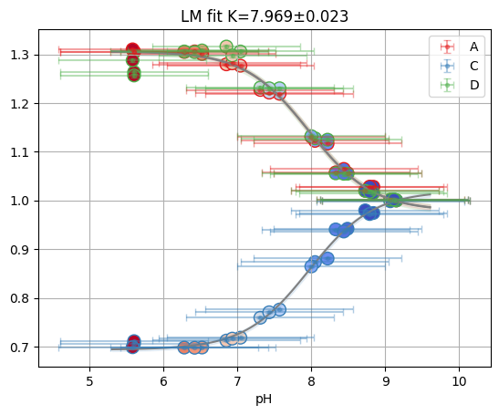
weight_multi_ds_titration(ds_svd)
res = fit_binding_glob(ds_svd)
res.figure

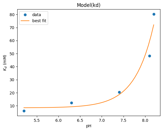
xx = np.array([5.2, 6.3, 7.4, 8.1, 8.2])
yy = np.array([6.05, 12.2, 20.38, 48.2, 80.3])


def kd(x, kd1, pka):
    return kd1 * (1 + 10 ** (pka - x)) / 10 ** (pka - x)


model = lmfit.Model(kd)
params = lmfit.Parameters()
params.add("kd1", value=10.0)
params.add("pka", value=6.6)
result = model.fit(yy, params, x=xx)

result.plot_fit(numpoints=50, ylabel="$K_d$ (mM)", xlabel="pH")

<Axes: title={'center': 'Model(kd)'}, xlabel='pH', ylabel='$K_d$ (mM)'>

import os

result_emcee = result.emcee(
    steps=int(os.environ.get("CLOPHFIT_DOCS_EMCEE_STEPS", "1800")),
    burn=int(os.environ.get("CLOPHFIT_DOCS_EMCEE_BURN", "150")),
    workers=int(os.environ.get("CLOPHFIT_EMCEE_WORKERS", "1")),
    nwalkers=int(os.environ.get("CLOPHFIT_DOCS_EMCEE_NWALKERS", "10")),
    seed=1,
    progress=False,
)
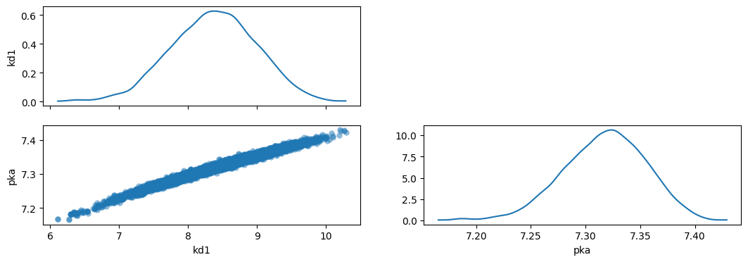
fig = plot_emcee(result_emcee.flatchain)

The chain is shorter than 50 times the integrated autocorrelation time for 2 parameter(s). Use this estimate with caution and run a longer chain!
N/50 = 6;
tau: [21.09140903 21.25484981]

import pymc as pm

# Assuming x_data and y_data are your data
with pm.Model() as model:
    kd1 = pm.Normal(
        "kd1", mu=result.params["kd1"].value, sigma=result.params["kd1"].stderr
    )
    pka = pm.Normal(
        "pka", mu=result.params["pka"].value, sigma=result.params["pka"].stderr
    )

    y_pred = pm.Deterministic("y_pred", kd(xx, kd1, pka))

    likelihood = pm.Normal("y", mu=y_pred, sigma=1, observed=yy)

    trace = pm.sample(1000, tune=2000, random_seed=1, chains=8, cores=8)

Initializing NUTS using jitter+adapt_diag...

Multiprocess sampling (8 chains in 8 jobs)

NUTS: [kd1, pka]

Sampling 8 chains for 2_000 tune and 1_000 draw iterations (16_000 + 8_000 draws total) took 27 seconds.

pm.model_to_graphviz(model)

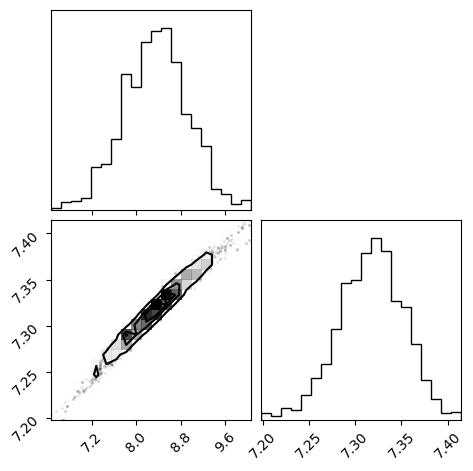
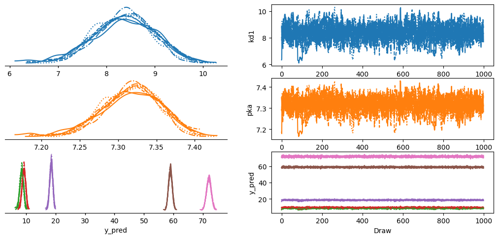
import arviz as az

az.plot_pair(trace, var_names=["kd1", "pka"], marginal=True, marginal_kind="kde")

<arviz_plots.plot_matrix.PlotMatrix at 0x79909ed54590>

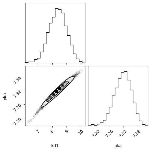
import corner

# Extract the posterior samples for the parameters of interest
kd1_samples = trace.posterior["kd1"].to_numpy().flatten()
pka_samples = trace.posterior["pka"].to_numpy().flatten()
samples_array = np.column_stack([kd1_samples, pka_samples])
# Plot the corner plot
f = corner.corner(samples_array, labels=["kd1", "pka"])

az.plot_trace_dist(trace)

<arviz_plots.plot_collection.PlotCollection at 0x79909306c6e0>

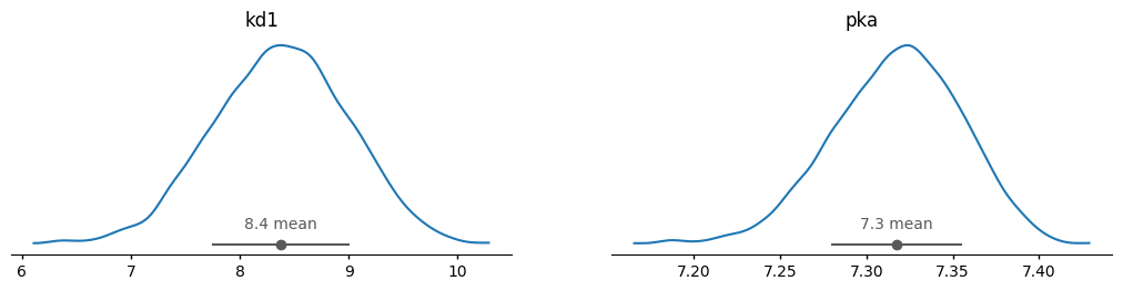
az.plot_dist(trace, var_names=["kd1", "pka"], ci_kind="eti", ci_prob=0.67)

<arviz_plots.plot_collection.PlotCollection at 0x799091a0b250>

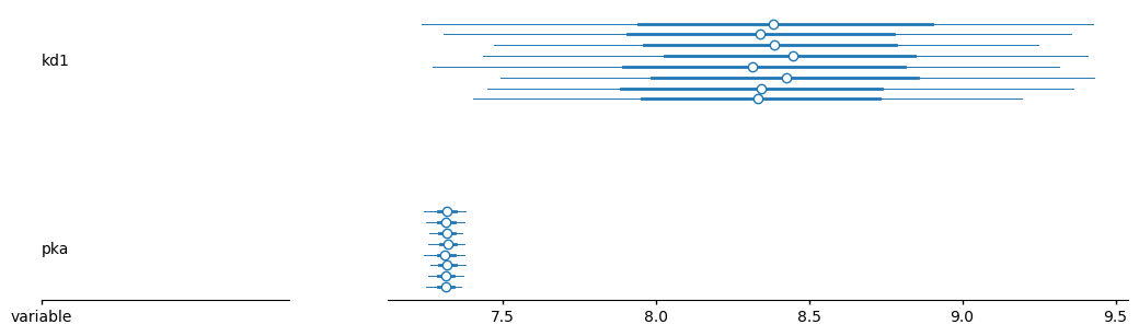
az.plot_forest(trace, var_names=["kd1", "pka"])
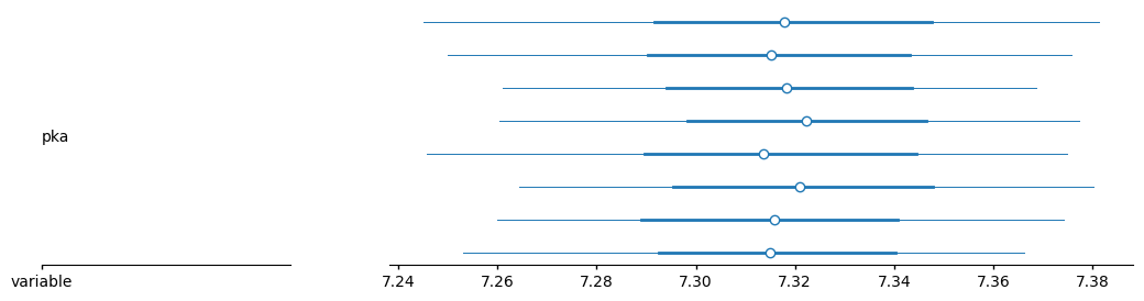
pm.plots.plot_forest(trace, var_names=["pka"])

<arviz_plots.plot_collection.PlotCollection at 0x79909322e3f0>