3. Getting started with prenspire#
[1]:
import random
from pathlib import Path
from clophfit.prenspire import prenspire

%load_ext autoreload
%autoreload 2
tpath = Path("../../tests/EnSpire")
[2]:
import pandas as pd
import numpy as np
import seaborn as sb
import matplotlib.pyplot as plt
[3]:
ef1 = prenspire.EnspireFile(tpath / "h148g-spettroC.csv")
ef2 = prenspire.EnspireFile(tpath / "e2-T-without_sample_column.csv")
ef3 = prenspire.EnspireFile(tpath / "24well_clop0_95.csv")
[4]:
ef3.wells, ef3._wells_platemap, ef3._platemap
[4]:
(['A03', 'A04', 'A05', 'A06', 'B01', 'B02', 'C01', 'C02', 'C03'],
 ['A03', 'A04', 'A05', 'A06', 'B01', 'B02', 'C01', 'C02', 'C03'],
 [['A', '  ', '  ', '- ', '- ', '- ', '- '],
  ['B', '- ', '- ', '  ', '  ', '  ', '  '],
  ['C', '- ', '- ', '- ', '  ', '  ', '  '],
  ['D', '  ', '  ', '  ', '  ', '  ', '  ']])
[5]:
ef1.__dict__.keys()
[5]:
dict_keys(['file', 'verbose', 'metadata', 'measurements', 'wells', '_ini', '_fin', '_wells_platemap', '_platemap'])
[6]:
ef1.measurements.keys(), ef2.measurements.keys()
[6]:
(dict_keys(['A']), dict_keys(['B', 'A', 'C', 'D', 'E', 'F', 'G', 'H']))
when testing each spectra for the presence of a single wavelength in the appropriate monochromator
[7]:
ef2.measurements["A"]["metadata"]
[7]:
{'temp': '25',
 'Monochromator': 'Excitation',
 'Min wavelength': '400',
 'Max wavelength': '510',
 'Wavelength': '530',
 'Using of excitation filter': 'Top',
 'Measurement height': '8.9',
 'Number of flashes': '50',
 'Number of flashes integrated': '50',
 'Flash power': '100'}
[8]:
ef2.measurements["A"].keys()
[8]:
dict_keys(['metadata', 'lambda', 'F01', 'F02', 'F03', 'F04', 'F05', 'F06', 'F07'])
[9]:
random.seed(11)
random.sample(ef1.measurements["A"]["F01"], 7)
[9]:
[2163.0, 607.0, 1846.0, 517.0, 572.0, 2145.0, 2028.0]
[10]:
en1 = prenspire.ExpNote(tpath / "h148g-spettroC-nota")
en1
[10]:
ExpNote(note_file=PosixPath('../../tests/EnSpire/h148g-spettroC-nota'), verbose=0, wells=['A01', 'A02', 'A03', 'A04', 'A05', 'A06', 'A07', 'A08', 'A09', 'A10', 'A11', 'B01', 'B02', 'B03', 'B04', 'B05', 'B06', 'B07', 'B08', 'B09', 'B10', 'B11', 'C01', 'C02', 'C03', 'C04', 'C05', 'C06', 'C07', 'C08', 'C09', 'C10', 'C11', 'D01', 'D02', 'D03', 'D04', 'D05', 'D06', 'D07', 'D08', 'D09', 'D10', 'D11', 'E01', 'E02', 'E03', 'E04', 'E05', 'E06', 'E07', 'E08', 'E09', 'E10', 'E11', 'F01', 'F02', 'F03', 'F04', 'F05', 'G01', 'G02', 'G03', 'G04', 'G05'], _note_list=[['Well', 'pH', 'Chloride'], ['A01', '5.2', '0'], ['A02', '5.2', '6.7'], ['A03', '5.2', '13.3'], ['A04', '5.2', '26.7'], ['A05', '5.2', '40'], ['A06', '5.2', '60'], ['A07', '5.2', '87'], ['A08', '5.2', '120'], ['A09', '5.2', '267'], ['A10', '5.2', '400'], ['A11', '5.2', '667'], ['B01', '6.3', '0'], ['B02', '6.3', '6.7'], ['B03', '6.3', '13.3'], ['B04', '6.3', '26.7'], ['B05', '6.3', '40'], ['B06', '6.3', '60'], ['B07', '6.3', '87'], ['B08', '6.3', '120'], ['B09', '6.3', '267'], ['B10', '6.3', '400'], ['B11', '6.3', '667'], ['C01', '7.4', '0'], ['C02', '7.4', '6.7'], ['C03', '7.4', '13.3'], ['C04', '7.4', '26.7'], ['C05', '7.4', '40'], ['C06', '7.4', '60'], ['C07', '7.4', '87'], ['C08', '7.4', '120'], ['C09', '7.4', '267'], ['C10', '7.4', '400'], ['C11', '7.4', '667'], ['D01', '8.1', '0'], ['D02', '8.1', '6.7'], ['D03', '8.1', '13.3'], ['D04', '8.1', '26.7'], ['D05', '8.1', '40'], ['D06', '8.1', '60'], ['D07', '8.1', '87'], ['D08', '8.1', '120'], ['D09', '8.1', '267'], ['D10', '8.1', '400'], ['D11', '8.1', '667'], ['E01', '8.2', '0'], ['E02', '8.2', '6.7'], ['E03', '8.2', '13.3'], ['E04', '8.2', '26.7'], ['E05', '8.2', '40'], ['E06', '8.2', '60'], ['E07', '8.2', '87'], ['E08', '8.2', '120'], ['E09', '8.2', '267'], ['E10', '8.2', '400'], ['E11', '8.2', '667'], ['F01', '5.2', 'buffer'], ['F02', '6.3', 'buffer'], ['F03', '7.4', 'buffer'], ['F04', '8.1', 'buffer'], ['F05', '8.2', 'buffer'], ['G01', '5.2', 'buffer'], ['G02', '6.3', 'buffer'], ['G03', '7.4', 'buffer'], ['G04', '8.1', 'buffer'], ['G05', '8.2', 'buffer']], titrations=[])
[11]:
ef = prenspire.EnspireFile(tpath / "G10.csv")
[12]:
en1.build_titrations(ef1)
en1.titrations[0].data["A"]
[12]:
| 5.2 | 6.3 | 7.4 | 8.1 | 8.2 | |
|---|---|---|---|---|---|
| A01 | B01 | C01 | D01 | E01 | |
| lambda | |||||
| 272.0 | 3151.0 | 4181.0 | 16413.0 | 29192.0 | 28816.0 |
| 273.0 | 3130.0 | 4204.0 | 16926.0 | 29909.0 | 29545.0 |
| 274.0 | 3043.0 | 4232.0 | 17331.0 | 30900.0 | 30750.0 |
| 275.0 | 3079.0 | 4283.0 | 17680.0 | 31717.0 | 31547.0 |
| 276.0 | 2975.0 | 4264.0 | 18020.0 | 32564.0 | 32336.0 |
| ... | ... | ... | ... | ... | ... |
| 496.0 | 636.0 | 4689.0 | 43230.0 | 87203.0 | 87842.0 |
| 497.0 | 683.0 | 4923.0 | 45173.0 | 89719.0 | 90666.0 |
| 498.0 | 632.0 | 4900.0 | 46725.0 | 93452.0 | 94101.0 |
| 499.0 | 854.0 | 5140.0 | 48452.0 | 96643.0 | 97506.0 |
| 500.0 | 573.0 | 5573.0 | 50025.0 | 99847.0 | 100715.0 |
229 rows × 5 columns
[13]:
fp = tpath / "h148g-spettroC-nota.csv"
n1 = prenspire.Note(fp, verbose=1)
n1.build_titrations(ef1)
Wells ['A02', 'A03']...['G04', 'G05'] generated.
[14]:
from clophfit.binding.fitting import analyze_spectra, analyze_spectra_glob

spectra = n1.titrations["H148G"][20.0]["Cl_0.0"]["A"]
[15]:
fp = tpath / "NTT-G10_note.csv"
nn = prenspire.Note(fp, verbose=1)
nn.build_titrations(ef)
Wells ['D02', 'D03']...['G07', 'G08'] generated.
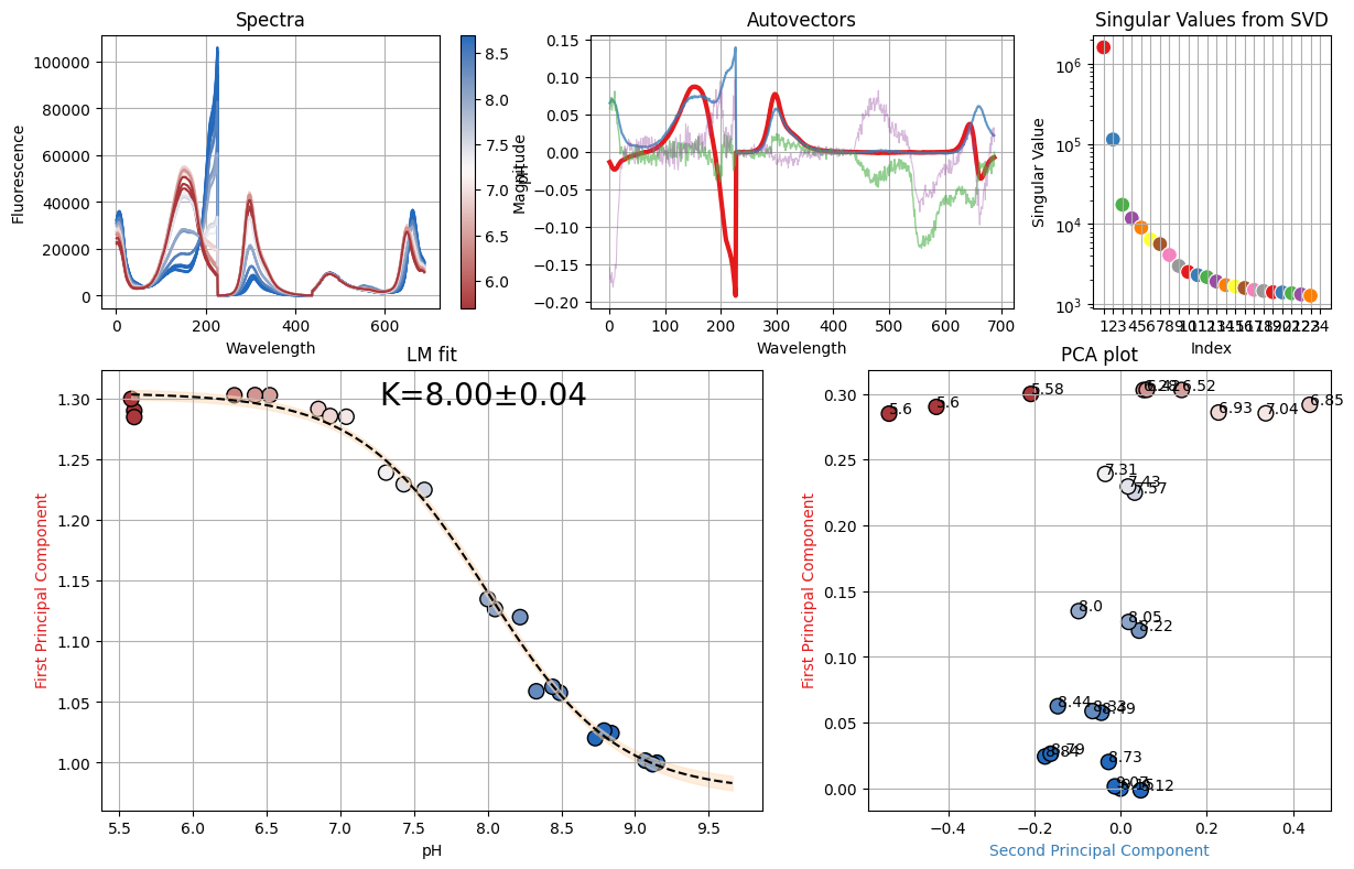
[16]:
titration = nn.titrations["NTT-G10"][20.0]["Cl_0.0"]
# titration = nn.titrations['NTT-G10'][37.0]['Cl_0.0']
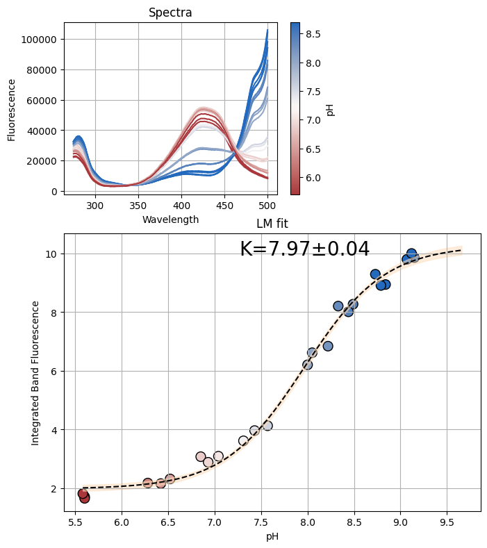
figures_results = analyze_spectra_glob(titration, "pH")
[17]:
figures_results
[17]:
(<Figure size 1200x800 with 6 Axes>,
 <lmfit.model.ModelResult at 0x7f31b026cee0>,
 None,
 None)
[18]:
print(figures_results[1].ci_report(ndigits=2, with_offset=False))
    99.73% 95.45% 68.27% _BEST_ 68.27% 95.45% 99.73%
 K :   7.87   7.92   7.96   8.00   8.04   8.08   8.13
 S1:   0.95   0.96   0.97   0.98   0.98   0.99   1.00
 S0:   1.29   1.30   1.30   1.30   1.31   1.31   1.32
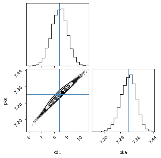
[19]:
import corner


def mcmc_sampling(result):
    # result = result.emcee(steps=500, burn=100, params=result.params, is_weighted=True)
    result = result.emcee(steps=500, burn=150)
    samples = result.flatchain
    return corner.corner(
        samples,
        labels=result.var_names,
        truths=list(result.params.valuesdict().values()),
    )


import lmfit

xx = np.array([5.2, 6.3, 7.4, 8.1, 8.2])
yy = np.array([6.05, 12.2, 20.38, 48.2, 80.3])


def kd(x, kd1, pka):
    return kd1 * (1 + 10 ** (pka - x)) / 10 ** (pka - x)


model = lmfit.Model(kd)
params = lmfit.Parameters()
params.add("kd1", value=10.0)
params.add("pka", value=6.6)

result = model.fit(yy, params, x=xx)

figure = mcmc_sampling(result)
100%|████████████████████████████████████████████████████████████████████████████████████████████████████████████████████████████████████████████████████████| 500/500 [00:05<00:00, 94.52it/s]
The chain is shorter than 50 times the integrated autocorrelation time for 2 parameter(s). Use this estimate with caution and run a longer chain!
N/50 = 10;
tau: [20.13286349 20.29655236]
[20]:
figure, result = analyze_spectra(
    nn.titrations["NTT-G10"][20.0]["Cl_0.0"]["C"], "pH", None
)
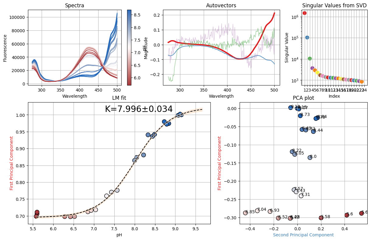
[21]:
spectra_A = nn.titrations["NTT-G10"][20.0]["Cl_0.0"]["A"]
spectra_C = nn.titrations["NTT-G10"][20.0]["Cl_0.0"]["C"]
spectra_D = nn.titrations["NTT-G10"][20.0]["Cl_0.0"]["D"]
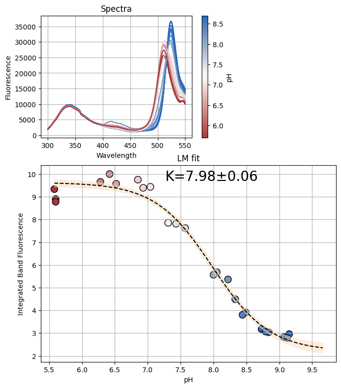
figA, resA = analyze_spectra(spectra_A, "pH", (466, 510))
figC, resC = analyze_spectra(spectra_C, "pH", (470, 500))
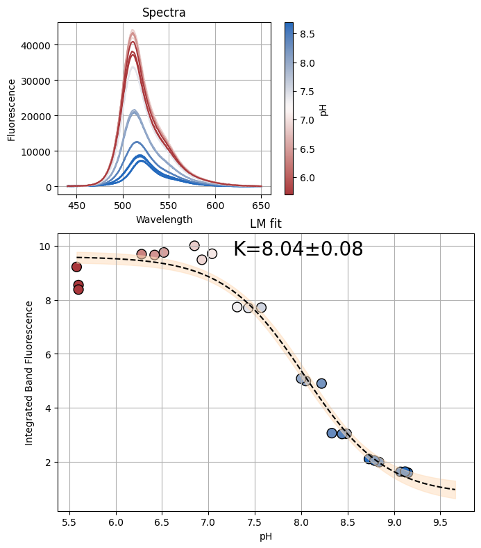
figD, resD = analyze_spectra(spectra_D, "pH", (450, 600))
# Combine the data from all datasets
x_combined = {"A": resA.userkws["x"], "C": resC.userkws["x"], "D": resD.userkws["x"]}
y_combined = {"A": resA.data, "C": resC.data, "D": resD.data}
[22]:
dbands = {"A": (466, 510), "C": (470, 500), "D": (450, 600)}
dbands = {
"A": (466, 510),
"C": (470, 500),
}
# dbands = {"A": (466, 510), }
# dbands = {}
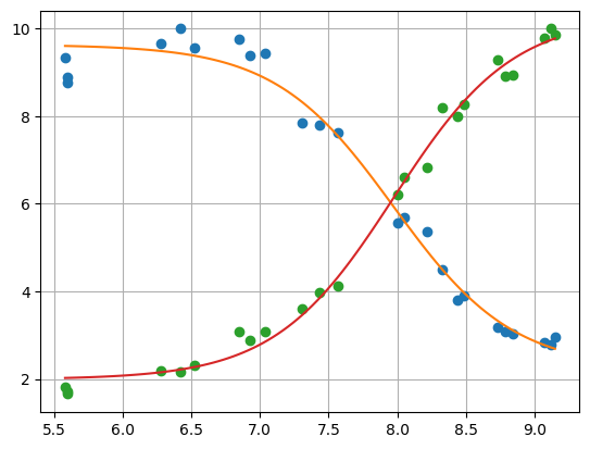
tup = analyze_spectra_glob(
nn.titrations["NTT-G10"][20.0]["Cl_0.0"], "pH", dbands, x_combined, y_combined
)
tup
[22]:
(None,
 None,
 <Figure size 640x480 with 1 Axes>,
 <lmfit.minimizer.MinimizerResult at 0x7f31725d0580>)
[23]:
tup[3]
[23]:
Fit Statistics
| fitting method | leastsq | |
| # function evals | 57 | |
| # data points | 48 | |
| # variables | 5 | |
| chi-square | 4.78487420 | |
| reduced chi-square | 0.11127614 | |
| Akaike info crit. | -100.675581 | |
| Bayesian info crit. | -91.3195763 |
Variables
| name | value | standard error | relative error | initial value | min | max | vary |
|---|---|---|---|---|---|---|---|
| K | 7.97506684 | 0.03667928 | (0.46%) | 7 | 0.00000000 | inf | True |
| S0_A | 9.63789512 | 0.11454433 | (1.19%) | 2.9567982827061576 | -inf | inf | True |
| S1_A | 2.22405960 | 0.16357651 | (7.35%) | 9.334882739985758 | -inf | inf | True |
| S0_C | 1.98809214 | 0.11679259 | (5.87%) | 9.858658373204044 | -inf | inf | True |
| S1_C | 10.2999977 | 0.17183986 | (1.67%) | 1.8147350421583364 | -inf | inf | True |
Correlations (unreported correlations are < 0.100)
| K | S1_C | +0.6776 |
| K | S1_A | -0.6349 |
| K | S0_C | +0.4319 |
| S1_A | S1_C | -0.4302 |
| K | S0_A | -0.3928 |
| S1_A | S0_C | -0.2742 |
| S0_A | S1_C | -0.2662 |
| S0_A | S0_C | -0.1696 |
[24]:
from clophfit.binding.fitting import _binding_residuals, _binding_pk
import lmfit

ndata = len(x_combined)
params = lmfit.Parameters()
params.add("K", value=5, min=0, max=10)
for label in x_combined:
    params.add(f"S0_{label}", value=y_combined[label][0])
    params.add(f"S1_{label}", value=y_combined[label][-1])
[25]:
result = lmfit.minimize(
    _binding_residuals, params, args=(_binding_pk, x_combined, y_combined)
)
result.params
[25]:
| name | value | standard error | relative error | initial value | min | max | vary |
|---|---|---|---|---|---|---|---|
| K | 8.00113658 | 0.03606111 | (0.45%) | 5 | 0.00000000 | 10.0000000 | True |
| S0_A | 9.60610648 | 0.13800935 | (1.44%) | 2.9567982827061576 | -inf | inf | True |
| S1_A | 2.14902484 | 0.19186866 | (8.93%) | 9.334882739985758 | -inf | inf | True |
| S0_C | 2.02401217 | 0.13975712 | (6.90%) | 9.858658373204044 | -inf | inf | True |
| S1_C | 10.3837396 | 0.19921960 | (1.92%) | 1.8147350421583364 | -inf | inf | True |
| S0_D | 9.65195727 | 0.14057651 | (1.46%) | 1.5932509691039798 | -inf | inf | True |
| S1_D | 0.89745241 | 0.20260476 | (22.58%) | 9.21780362986832 | -inf | inf | True |
[26]:
gmini = lmfit.Minimizer(
    _binding_residuals, params, fcn_args=(_binding_pk, x_combined, y_combined)
)
gres = gmini.minimize()

print(lmfit.conf_interval(gmini, gres, sigmas=[1])["K"])
[(0.6826894921370859, 7.965648370987939), (0.0, 8.001136579909678), (0.6826894921370859, 8.036541422589526)]
[27]:
en1._note_list

conc_well = [(line[1], line[0]) for line in en1._note_list if line[2] == "0"]
conc = [float(tpl[0]) for tpl in conc_well]
well = [tpl[1] for tpl in conc_well]
conc_well, conc, well
[27]:
([('5.2', 'A01'),
  ('6.3', 'B01'),
  ('7.4', 'C01'),
  ('8.1', 'D01'),
  ('8.2', 'E01')],
 [5.2, 6.3, 7.4, 8.1, 8.2],
 ['A01', 'B01', 'C01', 'D01', 'E01'])
[ ]:
@dataclass
class Metadata:

@dataclass
class Datum:
    well: str
    pH: float
    Cl: float
    T: float
    mut: str
    labels: list[str]
    metadata: dict[str, Metadata]
[21]:
en1.wells[:7]
[21]:
['A01', 'A02', 'A03', 'A04', 'A05', 'A06', 'A07']
[22]:
en1._note_list[:5]
[22]:
[['Well', 'pH', 'Chloride'],
 ['A01', '5.2', '0'],
 ['A02', '5.2', '6.7'],
 ['A03', '5.2', '13.3'],
 ['A04', '5.2', '26.7']]
[23]:
en1.wells == ef1.wells, en1.wells == ef2.wells
[23]:
(True, False)
[24]:
en1.build_titrations(ef1)
[14]:
en1.__dict__.keys()
[14]:
dict_keys(['note_file', 'verbose', 'wells', '_note_list', 'titrations', 'pH_values'])
[15]:
en1.pH_values
[15]:
['5.2', '6.3', '7.4', '8.1', '8.2']
[16]:
tit0 = en1.titrations[0]
tit3 = en1.titrations[3]
[17]:
tit0.__dict__.keys()
[17]:
dict_keys(['conc', 'data', 'cl'])
[18]:
tit0.conc, tit0.cl, tit3.conc, tit3.ph
[18]:
([5.2, 6.3, 7.4, 8.1, 8.2],
 '0',
 [0.0, 6.7, 13.3, 26.7, 40.0, 60.0, 87.0, 120.0, 267.0, 400.0, 667.0],
 '7.4')
[19]:
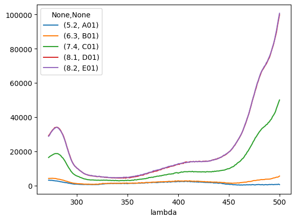
tit0.data["A"]
[19]:
| 5.2 | 6.3 | 7.4 | 8.1 | 8.2 | |
|---|---|---|---|---|---|
| A01 | B01 | C01 | D01 | E01 | |
| lambda | |||||
| 272.0 | 3151.0 | 4181.0 | 16413.0 | 29192.0 | 28816.0 |
| 273.0 | 3130.0 | 4204.0 | 16926.0 | 29909.0 | 29545.0 |
| 274.0 | 3043.0 | 4232.0 | 17331.0 | 30900.0 | 30750.0 |
| 275.0 | 3079.0 | 4283.0 | 17680.0 | 31717.0 | 31547.0 |
| 276.0 | 2975.0 | 4264.0 | 18020.0 | 32564.0 | 32336.0 |
| ... | ... | ... | ... | ... | ... |
| 496.0 | 636.0 | 4689.0 | 43230.0 | 87203.0 | 87842.0 |
| 497.0 | 683.0 | 4923.0 | 45173.0 | 89719.0 | 90666.0 |
| 498.0 | 632.0 | 4900.0 | 46725.0 | 93452.0 | 94101.0 |
| 499.0 | 854.0 | 5140.0 | 48452.0 | 96643.0 | 97506.0 |
| 500.0 | 573.0 | 5573.0 | 50025.0 | 99847.0 | 100715.0 |
229 rows × 5 columns
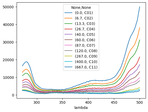
[20]:
tit0.plot()
[21]:
tit3.plot()