1. Fitting#
Requires:
r-4.1.3-1
1.1. Conventions and best approaches#
S0 Signal for unbound state
S1 Signal for bound state
K equilibrium constant (Kd or pKa)
order data from unbound to bound (e.g. cl: 0–>150 mM; pH 9–>5)
lmfit.Model has very convenient results plot functionalities and the unique possibility to estimate upper lower fitting curves.
R nls and nlsboot seems very convenient (Q-Q plt) and fast; nls can perform global fit but nlstools can not.
1.2. Initial imports#
import numpy as np
import scipy
import pandas as pd
import matplotlib.pyplot as plt
import seaborn as sb
import rpy2
from rpy2.robjects import r
from rpy2.robjects.packages import importr
from rpy2.robjects import globalenv
from rpy2.robjects import pandas2ri
import lmfit

pandas2ri.activate()
%load_ext rpy2.ipython

MASS = importr('MASS')
#r('library(MASS)')
The rpy2.ipython extension is already loaded. To reload it, use:
  %reload_ext rpy2.ipython
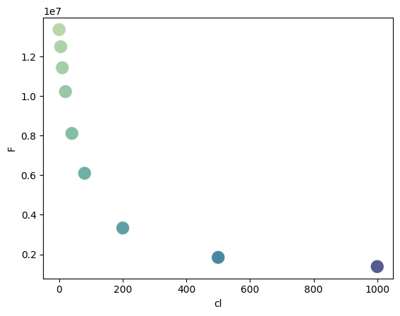
1.3. Single Cl titration.#
df = pd.read_table("../../tests/data/copyIP.txt")
sb.scatterplot(data=df, x="cl", y="F", hue=df.cl*df.F, palette="crest", s=200, alpha=.8, legend=False)
1.3.1. Using R#
d <- read.delim("../../tests/data/copyIP.txt")
fit = nls(F ~ (S0 + S1 * cl / Kd)/ (1 + cl / Kd), start = list(S0=7e7, S1=0, Kd=12), data=d)
summary(fit)
Formula: F ~ (S0 + S1 * cl/Kd)/(1 + cl/Kd)

Parameters:
    Estimate Std. Error t value Pr(>|t|)
S0 1.341e+07  8.713e+04 153.894 5.08e-12 ***
S1 5.635e+05  1.064e+05   5.296  0.00184 **
Kd 5.832e+01  2.247e+00  25.957 2.16e-07 ***
---
Signif. codes:  0 ‘***’ 0.001 ‘**’ 0.01 ‘*’ 0.05 ‘.’ 0.1 ‘ ’ 1

Residual standard error: 118200 on 6 degrees of freedom

Number of iterations to convergence: 6
Achieved convergence tolerance: 1.608e-06
confint(fit)
Waiting for profiling to be done...
           2.5%        97.5%
S0 1.319762e+07 1.362273e+07
S1 3.009078e+05 8.199737e+05
Kd 5.313128e+01 6.407096e+01
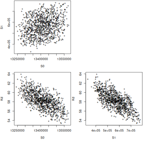
library(nlstools)
set.seed(4)
nb = nlsBoot(fit, niter=999)
summary(nb)
------
Bootstrap statistics
       Estimate   Std. error
S0 1.341194e+07 70877.210905
S1 5.662159e+05 88287.461199
Kd 5.827538e+01     1.834132

------
Median of bootstrap estimates and percentile confidence intervals
         Median         2.5%        97.5%
S0 1.341055e+07 1.328220e+07 1.354591e+07
S1 5.662406e+05 4.108650e+05 7.369380e+05
Kd 5.826980e+01 5.477262e+01 6.188986e+01
plot(nb)
1.3.2. using rpy2#
globalenv['Rdf'] = df

fit = rpy2.robjects.r('nls(F ~ (S0 + S1 * cl / Kd)/ (1 + cl / Kd), start = list(S0=7e7, S1=0, Kd=12), data=Rdf) ')
globalenv['rfit'] = fit
print(r.summary(fit))
print(r.confint(fit))
%R print("")
%R print(confint(rfit))
R[write to console]: Waiting for profiling to be done...

Formula: F ~ (S0 + S1 * cl/Kd)/(1 + cl/Kd)

Parameters:
    Estimate Std. Error t value Pr(>|t|)
S0 1.341e+07  8.713e+04 153.894 5.08e-12 ***
S1 5.635e+05  1.064e+05   5.296  0.00184 **
Kd 5.832e+01  2.247e+00  25.957 2.16e-07 ***
---
Signif. codes:  0 ‘***’ 0.001 ‘**’ 0.01 ‘*’ 0.05 ‘.’ 0.1 ‘ ’ 1

Residual standard error: 118200 on 6 degrees of freedom

Number of iterations to convergence: 6
Achieved convergence tolerance: 1.608e-06


[[1.31976181e+07 1.36227292e+07]
 [3.00907829e+05 8.19973684e+05]
 [5.31312807e+01 6.40709639e+01]]
[1] ""
R[write to console]: Waiting for profiling to be done...
           2.5%        97.5%
S0 1.319762e+07 1.362273e+07
S1 3.009078e+05 8.199737e+05
Kd 5.313128e+01 6.407096e+01
array([[1.31976181e+07, 1.36227292e+07],
       [3.00907829e+05, 8.19973684e+05],
       [5.31312807e+01, 6.40709639e+01]])
With older versions Rpy2 output looked nicer
print(MASS.confint_nls(fit, 'Kd'))
print(rpy2.robjects.r('summary(rfit)'))
R[write to console]: Waiting for profiling to be done...
[53.13128065 64.07096394]

Formula: F ~ (S0 + S1 * cl/Kd)/(1 + cl/Kd)

Parameters:
    Estimate Std. Error t value Pr(>|t|)
S0 1.341e+07  8.713e+04 153.894 5.08e-12 ***
S1 5.635e+05  1.064e+05   5.296  0.00184 **
Kd 5.832e+01  2.247e+00  25.957 2.16e-07 ***
---
Signif. codes:  0 ‘***’ 0.001 ‘**’ 0.01 ‘*’ 0.05 ‘.’ 0.1 ‘ ’ 1

Residual standard error: 118200 on 6 degrees of freedom

Number of iterations to convergence: 6
Achieved convergence tolerance: 1.608e-06
nlstools = importr('nlstools')
base = importr('base')
base.set_seed(4)
nb = nlstools.nlsBoot(fit, niter=999)
globalenv['nb'] = nb
globalenv['fit'] = fit
%%R
plot(nb)
summary(nb)
------
Bootstrap statistics
       Estimate   Std. error
S0 1.341194e+07 70877.210905
S1 5.662159e+05 88287.461199
Kd 5.827538e+01     1.834132

------
Median of bootstrap estimates and percentile confidence intervals
         Median         2.5%        97.5%
S0 1.341055e+07 1.328220e+07 1.354591e+07
S1 5.662406e+05 4.108650e+05 7.369380e+05
Kd 5.826980e+01 5.477262e+01 6.188986e+01

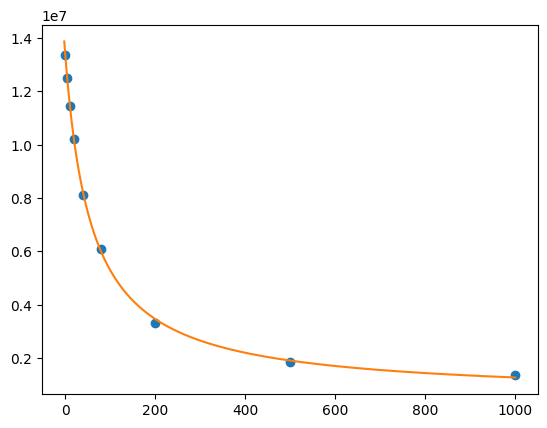
1.3.3. lmfit#
import lmfit

def residual(pars, x, y=None):
    S0 =  pars['S0']
    S1 =  pars['S1']
    Kd = pars['Kd']
    model = (S0 + S1 * x / Kd) / (1 + x / Kd)
    if y is None:
        return model
    return (y - model)

params = lmfit.Parameters()
params.add('S0', value=df.F[0])
params.add('S1', value=100)
params.add('Kd', value=50, vary=True)

out = lmfit.minimize(residual, params, args=(df.cl, df.F,))

xdelta = (df.cl.max() - df.cl.min()) / 500
xfit = np.arange(df.cl.min() - xdelta, df.cl.max() + xdelta, xdelta)
yfit = residual(out.params, xfit)
print(lmfit.fit_report(out.params))
plt.plot(df.cl, df.F, "o", xfit, yfit, "-")
[[Variables]]
    S0:  13408867.7 +/- 87130.4207 (0.65%) (init = 1.33579e+07)
    S1:  563536.896 +/- 106411.773 (18.88%) (init = 100)
    Kd:  58.3187813 +/- 2.24670302 (3.85%) (init = 50)
[[Correlations]] (unreported correlations are < 0.100)
    C(S1, Kd) = -0.712
    C(S0, Kd) = -0.656
    C(S0, S1) = 0.275
import lmfit
def residuals(p):
    S0 =  p['S0']
    S1 =  p['S1']
    Kd = p['Kd']
    model = (S0 + S1 * df.cl / Kd) / (1 + df.cl / Kd)
    return (model - df.F)

mini = lmfit.Minimizer(residuals, params)
res = mini.minimize()
ci, tr = lmfit.conf_interval(mini, res, sigmas=[.68, .95], trace=True)
print(lmfit.ci_report(ci, with_offset=False, ndigits=2))
print(lmfit.fit_report(res, show_correl=False, sort_pars=True))
    95.00% 68.00% _BEST_ 68.00% 95.00%
 S0:13197616.3413314946.3513408867.6813503300.3813622729.13
 S1:300911.47447991.63563536.93677869.66819977.61
 Kd:  53.13  55.96  58.32  60.79  64.07
[[Fit Statistics]]
    # fitting method   = leastsq
    # function evals   = 17
    # data points      = 9
    # variables        = 3
    chi-square         = 8.3839e+10
    reduced chi-square = 1.3973e+10
    Akaike info crit   = 212.594471
    Bayesian info crit = 213.186145
[[Variables]]
    Kd:  58.3187808 +/- 2.24670301 (3.85%) (init = 50)
    S0:  13408867.7 +/- 87130.4216 (0.65%) (init = 1.33579e+07)
    S1:  563536.932 +/- 106411.771 (18.88%) (init = 100)
names = res.params.keys()
i = 0
gs = plt.GridSpec(4, 4)
sx = {}
sy = {}
for fixed in names:
    j = 0
    for free in names:
        if j in sx and i in sy:
            ax = plt.subplot(gs[i, j], sharex=sx[j], sharey=sy[i])
        elif i in sy:
            ax = plt.subplot(gs[i, j], sharey=sy[i])
            sx[j] = ax
        elif j in sx:
            ax = plt.subplot(gs[i, j], sharex=sx[j])
            sy[i] = ax
        else:
            ax = plt.subplot(gs[i, j])
            sy[i] = ax
            sx[j] = ax
        if i < 3:
            plt.setp(ax.get_xticklabels(), visible=True)
        else:
            ax.set_xlabel(free)

        if j > 0:
            plt.setp(ax.get_yticklabels(), visible=False)
        else:
            ax.set_ylabel(fixed)

        rest = tr[fixed]
        prob = rest['prob']
        f = prob < 0.96

        x, y = rest[free], rest[fixed]
        ax.scatter(x[f], y[f], c=1-prob[f], s=25*(1-prob[f]+0.5))
        ax.autoscale(1, 1)
        j += 1
    i += 1
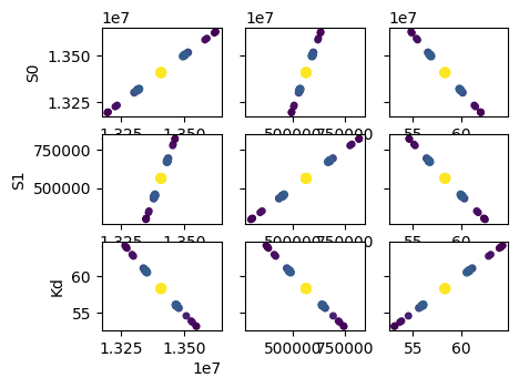
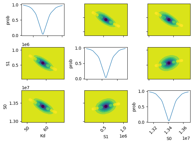
names = list(res.params.keys())

plt.figure()
for i in range(3):
    for j in range(3):
        indx = 9-j*3-i
        ax = plt.subplot(3, 3, indx)
        ax.ticklabel_format(style='sci', scilimits=(-2, 2), axis='y')

        # set-up labels and tick marks
        ax.tick_params(labelleft=False, labelbottom=False)
        if indx in (1, 4, 7):
            plt.ylabel(names[j])
            ax.tick_params(labelleft=True)
        if indx == 1:
            ax.tick_params(labelleft=True)
        if indx in (7, 8, 9):
            plt.xlabel(names[i])
            ax.tick_params(labelbottom=True)
            [label.set_rotation(45) for label in ax.get_xticklabels()]

        if i != j:
            x, y, m = lmfit.conf_interval2d(mini, res, names[i], names[j], 20, 20)
            plt.contourf(x, y, m, np.linspace(0, 1, 10))

            x = tr[names[i]][names[i]]
            y = tr[names[i]][names[j]]
            pr = tr[names[i]]['prob']
            s = np.argsort(x)
            plt.scatter(x[s], y[s], c=pr[s], s=30, lw=1)

        else:
            x = tr[names[i]][names[i]]
            y = tr[names[i]]['prob']

            t, s = np.unique(x, True)
            f = scipy.interpolate.interp1d(t, y[s], 'slinear')
            xn = np.linspace(x.min(), x.max(), 50)
            plt.plot(xn, f(xn), lw=1)
            plt.ylabel('prob')
            ax.tick_params(labelleft=True)

plt.tight_layout()
lmfit.report_fit(out.params, min_correl=0.25)
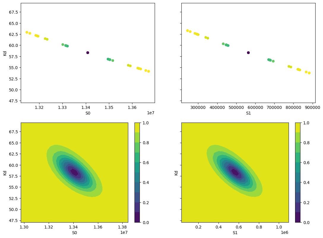
ci, trace = lmfit.conf_interval(mini, res, sigmas=[1, 2], trace=True)
lmfit.printfuncs.report_ci(ci)
fig, axes = plt.subplots(2, 2, figsize=(12.8, 9.6), sharey=True)
cx1, cy1, prob = trace['S0']['S0'], trace['S0']['Kd'], trace['S0']['prob']
cx2, cy2, prob2 = trace['S1']['S1'], trace['S1']['Kd'], trace['S1']['prob']
axes[0][0].scatter(cx1, cy1, c=prob, s=30)
axes[0][0].set_xlabel('S0')
axes[0][0].set_ylabel('Kd')
axes[0][1].scatter(cx2, cy2, c=prob2, s=30)
axes[0][1].set_xlabel('S1')
cx, cy, grid = lmfit.conf_interval2d(mini, res, 'S0', 'Kd', 30, 30)
ctp = axes[1][0].contourf(cx, cy, grid, np.linspace(0, 1, 11))
fig.colorbar(ctp, ax=axes[1][0])
axes[1][0].set_xlabel('S0')
axes[1][0].set_ylabel('Kd')
cx, cy, grid = lmfit.conf_interval2d(mini, res, 'S1', 'Kd', 30, 30)
ctp = axes[1][1].contourf(cx, cy, grid, np.linspace(0, 1, 11))
fig.colorbar(ctp, ax=axes[1][1])
axes[1][1].set_xlabel('S1')
axes[1][1].set_ylabel('Kd')
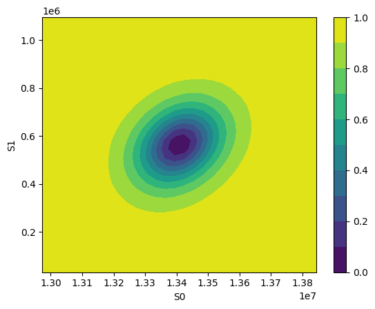
x, y, grid = lmfit.conf_interval2d(mini, res, 'S0','S1', 30, 30)
plt.contourf(x, y, grid, np.linspace(0,1,11))
plt.xlabel('S0')
plt.colorbar()
plt.ylabel('S1')
[[Variables]]
    S0:  13408867.7 +/- 87130.4207 (0.65%) (init = 1.33579e+07)
    S1:  563536.896 +/- 106411.773 (18.88%) (init = 100)
    Kd:  58.3187813 +/- 2.24670302 (3.85%) (init = 50)
[[Correlations]] (unreported correlations are < 0.250)
    C(S1, Kd) = -0.712
    C(S0, Kd) = -0.656
    C(S0, S1) = 0.275
       95.45%    68.27%    _BEST_    68.27%    95.45%
 S0:-217226.57750-94491.3408813408867.68157+95008.90246+219989.07757
 S1:-270193.18488-116251.92509563536.93239+115024.55042+263650.95181
 Kd:  -5.32812  -2.37783  58.31878  +2.48963  +5.92424
1.4. Notes#
You could implement global fitting using scipy.leastq but will sometime fail in bootstrapping. lmfit resulted much more robust
def fit_pH_global(fz, x, dy1, dy2):
    """Fit 2 dataset (x, y1, y2) with a single protonation site model
    """
    y1 = np.array(dy1)
    y2 = np.array(dy2)

    def ssq(p, x, y1, y2):
        return np.r_[y1 - fz(p[0], p[1:3], x), y2 - fz(p[0], p[3:5], x)]
    p0 = np.r_[x[2], y1[0], y1[-1], y2[0], y2[-1]]
    p, cov, info, msg, success = optimize.leastsq(ssq, p0, args=(x, y1, y2),
                                                  full_output=True, xtol=1e-11)
    res = namedtuple("Result", "success msg df chisqr K sK SA_1 sSA_1 \
                     SB_1 sSB_1 SA_2 sSA_2 SB_2 sSB_2")
    res.msg = msg
    res.success = success
    if 1 <= success <= 4:
        chisq = sum(info['fvec'] * info['fvec'])
        res.df = len(y1) + len(y2) - len(p)
        res.chisqr = chisq / res.df
        res.K = p[0]
        #res.sK = np.sqrt(cov[0][0] * res.chisqr)
        res.SA_1 = p[1]
        #res.sSA_1 = np.sqrt(cov[1][1] * res.chisqr)
        res.SB_1 = p[2]
        #res.sSB_1 = np.sqrt(cov[2][2] * res.chisqr)
        res.SA_2 = p[3]
        #res.sSA_2 = np.sqrt(cov[3][3] * res.chisqr)
        res.SB_2 = p[4]
        #res.sSB_2 = np.sqrt(cov[4][4] * res.chisqr)
    return res

result = fit_pH_global(fz, df.x, df.y1, df.y2)