3. Getting started with prenspire#
[1]:
import random
from pathlib import Path
from clophfit.prenspire import prenspire

%load_ext autoreload
%autoreload 2
tpath = Path("../../tests/EnSpire")
[2]:
import pandas as pd
import numpy as np
import seaborn as sb
import matplotlib.pyplot as plt
import arviz as az
import lmfit

from clophfit.binding.fitting import (
    analyze_spectra,
    analyze_spectra_glob,
    Dataset,
    fit_binding_glob,
)
from clophfit.binding.plotting import plot_emcee, plot_emcee_k_on_ax
from clophfit.__main__ import _print_result
[3]:
ef1 = prenspire.EnspireFile(tpath / "h148g-spettroC.csv")
ef2 = prenspire.EnspireFile(tpath / "e2-T-without_sample_column.csv")
ef3 = prenspire.EnspireFile(tpath / "24well_clop0_95.csv")
[4]:
ef3.wells, ef3._wells_platemap, ef3._platemap
[4]:
(['A03', 'A04', 'A05', 'A06', 'B01', 'B02', 'C01', 'C02', 'C03'],
 ['A03', 'A04', 'A05', 'A06', 'B01', 'B02', 'C01', 'C02', 'C03'],
 [['A', '  ', '  ', '- ', '- ', '- ', '- '],
  ['B', '- ', '- ', '  ', '  ', '  ', '  '],
  ['C', '- ', '- ', '- ', '  ', '  ', '  '],
  ['D', '  ', '  ', '  ', '  ', '  ', '  ']])
[5]:
ef1.__dict__.keys()
[5]:
dict_keys(['file', 'verbose', 'metadata', 'measurements', 'wells', '_ini', '_fin', '_wells_platemap', '_platemap'])
[6]:
ef1.measurements.keys(), ef2.measurements.keys()
[6]:
(dict_keys(['A']), dict_keys(['B', 'A', 'C', 'D', 'E', 'F', 'G', 'H']))
when testing each spectra for the presence of a single wavelength in the appropriate monochromator
[7]:
ef2.measurements["A"]["metadata"]
[7]:
{'temp': '25',
 'Monochromator': 'Excitation',
 'Min wavelength': '400',
 'Max wavelength': '510',
 'Wavelength': '530',
 'Using of excitation filter': 'Top',
 'Measurement height': '8.9',
 'Number of flashes': '50',
 'Number of flashes integrated': '50',
 'Flash power': '100'}
[8]:
ef2.measurements["A"].keys()
[8]:
dict_keys(['metadata', 'lambda', 'F01', 'F02', 'F03', 'F04', 'F05', 'F06', 'F07'])
[9]:
random.seed(11)
random.sample(ef1.measurements["A"]["F01"], 7)
[9]:
[2163.0, 607.0, 1846.0, 517.0, 572.0, 2145.0, 2028.0]
[10]:
fp = tpath / "h148g-spettroC-nota.csv"
n1 = prenspire.Note(fp, verbose=1)
n1._note.set_index("Well").loc["A01", ["Name", "Temp"]]
Wells ['A01', 'A02']...['G04', 'G05'] generated.
[10]:
Name    H148G
Temp     20.0
Name: A01, dtype: object
[11]:
n1.__dict__.keys()
[11]:
dict_keys(['fpath', 'verbose', 'wells', '_note', 'titrations'])
[12]:
n1.wells == ef1.wells, n1.wells == ef2.wells
[12]:
(True, False)
[13]:
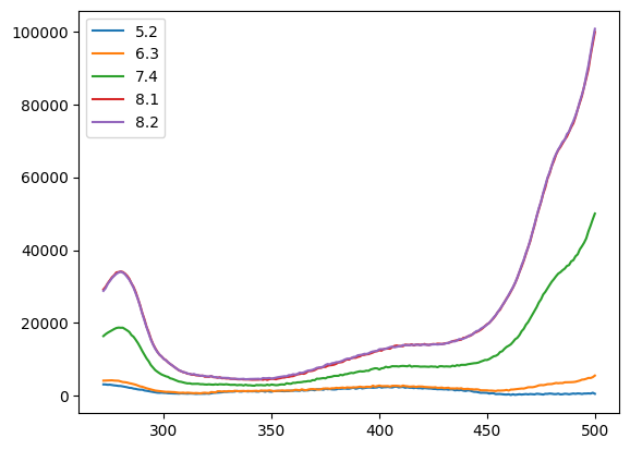
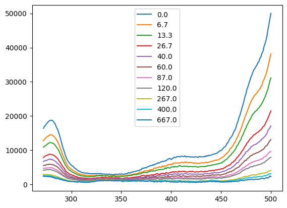
n1.build_titrations(ef1)
tit0 = n1.titrations["H148G"][20.0]["Cl_0.0"]["A"]
tit3 = n1.titrations["H148G"][20.0]["pH_7.4"]["A"]
tit0
[13]:
| 5.2 | 6.3 | 7.4 | 8.1 | 8.2 | |
|---|---|---|---|---|---|
| 272.0 | 3151.0 | 4181.0 | 16413.0 | 29192.0 | 28816.0 |
| 273.0 | 3130.0 | 4204.0 | 16926.0 | 29909.0 | 29545.0 |
| 274.0 | 3043.0 | 4232.0 | 17331.0 | 30900.0 | 30750.0 |
| 275.0 | 3079.0 | 4283.0 | 17680.0 | 31717.0 | 31547.0 |
| 276.0 | 2975.0 | 4264.0 | 18020.0 | 32564.0 | 32336.0 |
| ... | ... | ... | ... | ... | ... |
| 496.0 | 636.0 | 4689.0 | 43230.0 | 87203.0 | 87842.0 |
| 497.0 | 683.0 | 4923.0 | 45173.0 | 89719.0 | 90666.0 |
| 498.0 | 632.0 | 4900.0 | 46725.0 | 93452.0 | 94101.0 |
| 499.0 | 854.0 | 5140.0 | 48452.0 | 96643.0 | 97506.0 |
| 500.0 | 573.0 | 5573.0 | 50025.0 | 99847.0 | 100715.0 |
229 rows × 5 columns
[14]:
tit0.plot()
tit3.plot()
[14]:
<Axes: >
[ ]:
@dataclass
class Metadata:

@dataclass
class Datum:
    well: str
    pH: float
    Cl: float
    T: float
    mut: str
    labels: list[str]
    metadata: dict[str, Metadata]
[15]:
ef = prenspire.EnspireFile(tpath / "G10.csv")
fp = tpath / "NTT-G10_note.csv"
nn = prenspire.Note(fp, verbose=1)
nn.build_titrations(ef)
spectra = nn.titrations["NTT-G10"][20.0]["Cl_0.0"]["C"]
Wells ['D01', 'D02']...['G07', 'G08'] generated.
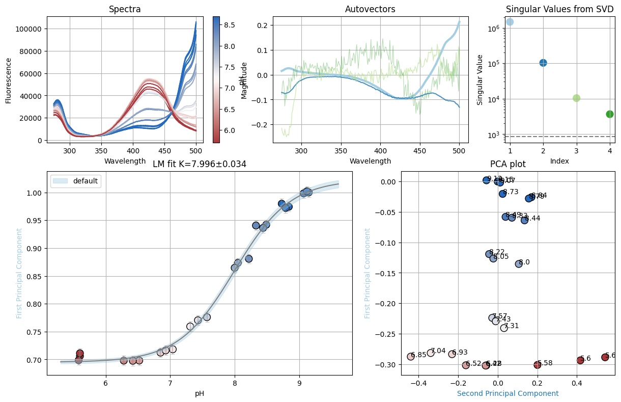
[16]:
f_res = analyze_spectra(spectra, is_ph=True, band=None)
print(f_res.result.chisqr)
plt.show()
f_res.figure
23.999999999999904
[16]:
[17]:
def dataset_from_lres(lkey, lres, is_ph):
    x, y = {}, {}
    for k, res in zip(lkey, lres):
        x[k] = res.mini.userargs[0]["default"].x
        y[k] = res.mini.userargs[0]["default"].y
    return Dataset(x, y, is_ph)


spectra_A = nn.titrations["NTT-G10"][20.0]["Cl_0.0"]["A"]
spectra_C = nn.titrations["NTT-G10"][20.0]["Cl_0.0"]["C"]
spectra_D = nn.titrations["NTT-G10"][20.0]["Cl_0.0"]["D"]

resA = analyze_spectra(spectra_A, "pH", (466, 510))
resC = analyze_spectra(spectra_C, "pH", (470, 500))
resD = analyze_spectra(spectra_D, "pH", (450, 600))
ds_bands = dataset_from_lres(["A", "C", "D"], [resA, resC, resD], True)

resA = analyze_spectra(spectra_A, "pH")
resC = analyze_spectra(spectra_C, "pH")
resD = analyze_spectra(spectra_D, "pH")
ds_svd = dataset_from_lres(["A", "C", "D"], [resA, resC, resD], True)
[18]:
dbands = {"D": (466, 510)}
tit = nn.titrations["NTT-G10"][20.0]["Cl_0.0"]
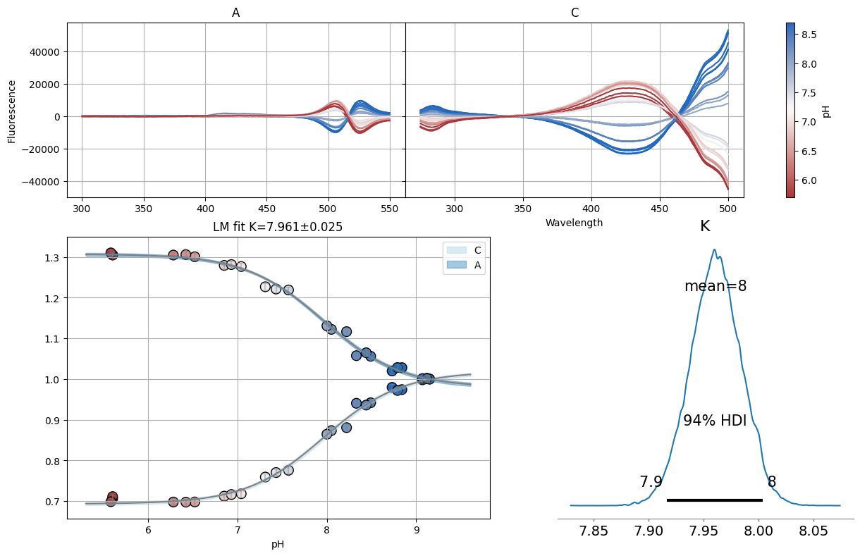
sgres = analyze_spectra_glob(tit, ds_svd, dbands)
sgres.svd.figure
sgres.gsvd.figure
100%|██████████████████████████████████████████████████████████████████████████████████████████████████████████████████████████████████████████████████████| 1800/1800 [00:27<00:00, 66.20it/s]
The chain is shorter than 50 times the integrated autocorrelation time for 5 parameter(s). Use this estimate with caution and run a longer chain!
N/50 = 36;
tau: [52.75761592 45.7772326  55.71405633 41.88746234 42.93106298]
[18]:
[19]:
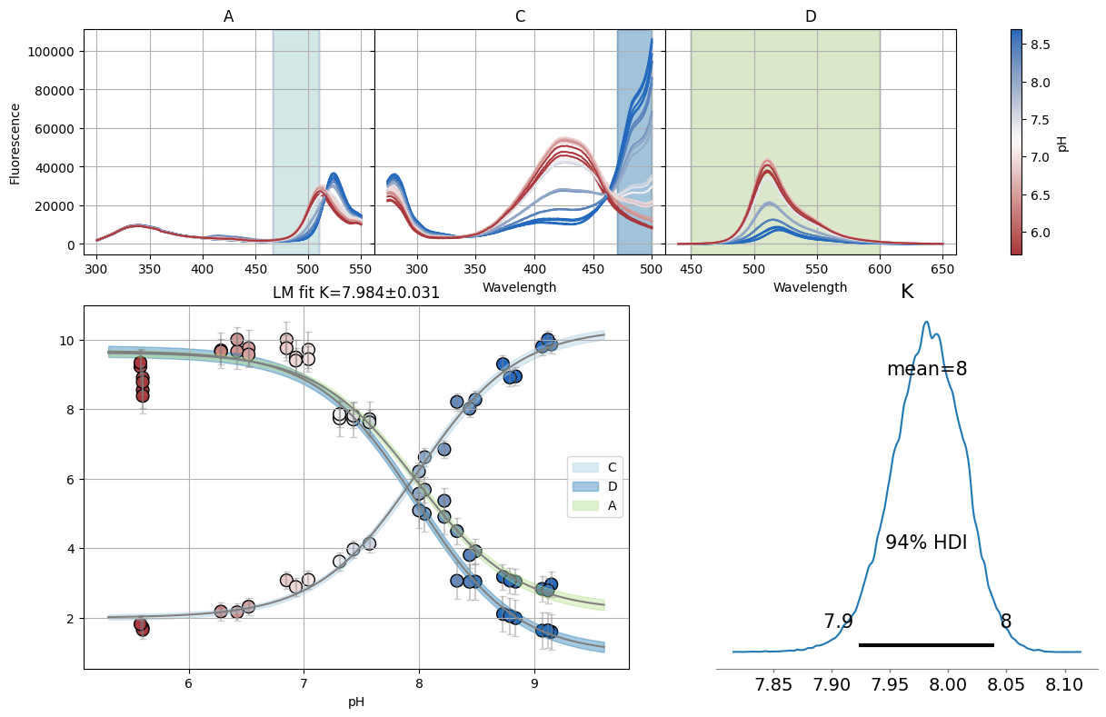
dbands = {"A": (466, 510), "C": (470, 500), "D": (450, 600)}
sgres = analyze_spectra_glob(nn.titrations["NTT-G10"][20.0]["Cl_0.0"], ds_bands, dbands)
sgres.bands.figure
100%|██████████████████████████████████████████████████████████████████████████████████████████████████████████████████████████████████████████████████████| 1800/1800 [00:32<00:00, 55.68it/s]
The chain is shorter than 50 times the integrated autocorrelation time for 7 parameter(s). Use this estimate with caution and run a longer chain!
N/50 = 36;
tau: [60.3414749  59.02308364 82.43868974 64.34312466 77.15823087 58.71136724
 55.94448519]
[19]:
[20]:
ci = lmfit.conf_interval(sgres.bands.mini, sgres.bands.result)
print(lmfit.ci_report(ci, ndigits=2, with_offset=False))
      99.73% 95.45% 68.27% _BEST_ 68.27% 95.45% 99.73%
 S0_C:   9.90  10.05  10.19  10.33  10.47  10.62  10.79
 S1_C:   1.70   1.81   1.91   2.00   2.10   2.19   2.29
 S0_D:   0.21   0.47   0.72   0.96   1.19   1.42   1.67
 S1_D:   9.12   9.31   9.50   9.68   9.85  10.04  10.23
 S0_A:   1.65   1.84   2.02   2.20   2.37   2.54   2.72
 S1_A:   9.23   9.37   9.50   9.63   9.76   9.89  10.03
 K   :   7.89   7.92   7.95   7.98   8.02   8.05   8.08
[21]:
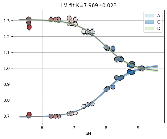
res = fit_binding_glob(ds_svd, True)
res.figure
[21]:
[22]:
xx = np.array([5.2, 6.3, 7.4, 8.1, 8.2])
yy = np.array([6.05, 12.2, 20.38, 48.2, 80.3])
def kd(x, kd1, pka):
return kd1 * (1 + 10 ** (pka - x)) / 10 ** (pka - x)
model = lmfit.Model(kd)
params = lmfit.Parameters()
params.add("kd1", value=10.0)
params.add("pka", value=6.6)
result = model.fit(yy, params, x=xx)
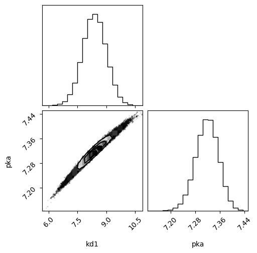
result_emcee = result.emcee(steps=1800, burn=150)
plot_emcee(result_emcee)
100%|██████████████████████████████████████████████████████████████████████████████████████████████████████████████████████████████████████████████████████| 1800/1800 [00:21<00:00, 83.69it/s]
[22]:
(<Figure size 550x550 with 4 Axes>, [])